How to Extract Market-Implied Probability Distributions from Options Using Python

7/9/2025

Introduction

Financial markets are driven by expectations. Every moment, millions of market participants collectively form views on future asset prices, based on fundamentals, technical patterns, macroeconomic indicators, or sentiment. While these views are not directly observable, they are indirectly embedded in the prices of derivatives, especially options. Options are contracts that derive their value from the expected behavior of an underlying asset, making them a rich source of information about market expectations.

One of the most powerful tools for revealing these embedded expectations is the implied probability density function (PDF). Unlike a forecast that gives a single price target, a PDF describes the full spectrum of possible outcomes and their likelihoods as perceived by the market. Extracting this market-implied PDF from option prices provides a probabilistic lens through which investors and analysts can understand expected volatility, tail risks, skewness, and the probability of extreme events.

This article serves as a comprehensive, step-by-step guide to extracting such implied PDFs using real market data. We blend theoretical foundations with a hands-on Python implementation that uses Yahoo Finance data to construct the PDF. Every step is motivated by financial intuition and mathematical rigor, ensuring a clear understanding of both how and why the process works.

Theoretical Background

Risk-Neutral Valuation

Before deriving implied PDFs, we need to understand the framework in which option prices are interpreted: the risk-neutral measure. In this mathematical construct, we price assets as though investors are indifferent to risk. While this is a simplification of reality, it allows us to treat current option prices as the discounted expected value of their future payoffs:

$C(K) = e^{-rt}\mathbb{E}^Q[(S_t - K)^+]$

Where:

$C(K)$ is the premium of a European call option with strike $K$
$r$ is the risk-free interest rate
$t$ is time to maturity
$S_t$ is the underlying asset price at maturity
$\mathbb{E}^Q$ is the expectation under the risk-neutral probability measure $Q$

This risk-neutral perspective is foundational for derivative pricing. It allows us to reverse-engineer market expectations by assuming that today's prices already incorporate a fair valuation of all future states, adjusted only by the time value of money.

Breeden-Litzenberger Formula

In 1978, Breeden and Litzenberger showed that if call prices are smooth and continuous with respect to strike, the second derivative of the call price with respect to strike gives us the risk-neutral probability density function:

$f(K) = e^{rt} \frac{\partial^2 C(K)}{\partial K^2}$

This elegant formula is the bridge between observed option prices and the market's implied beliefs. Once we compute this second derivative, we directly uncover the shape of the distribution of future prices implied by the market.

Implementing the Black-Scholes Model in Python

The Black-Scholes model gives the theoretical price of European call options under the assumption of log-normal asset returns and constant volatility:

from scipy.stats import norm
import numpy as np

def call_value(S, K, sigma, t, r=0):
    with np.errstate(divide='ignore'):
        d1 = (np.log(S/K) + (r + 0.5*sigma**2)*t) / (sigma*np.sqrt(t))
        d2 = d1 - sigma*np.sqrt(t)
    return S*norm.cdf(d1) - K*np.exp(-r*t)*norm.cdf(d2)

This function is essential for computing the theoretical value of options for given volatility levels. Later, we invert this process to extract the volatility that matches observed market prices.

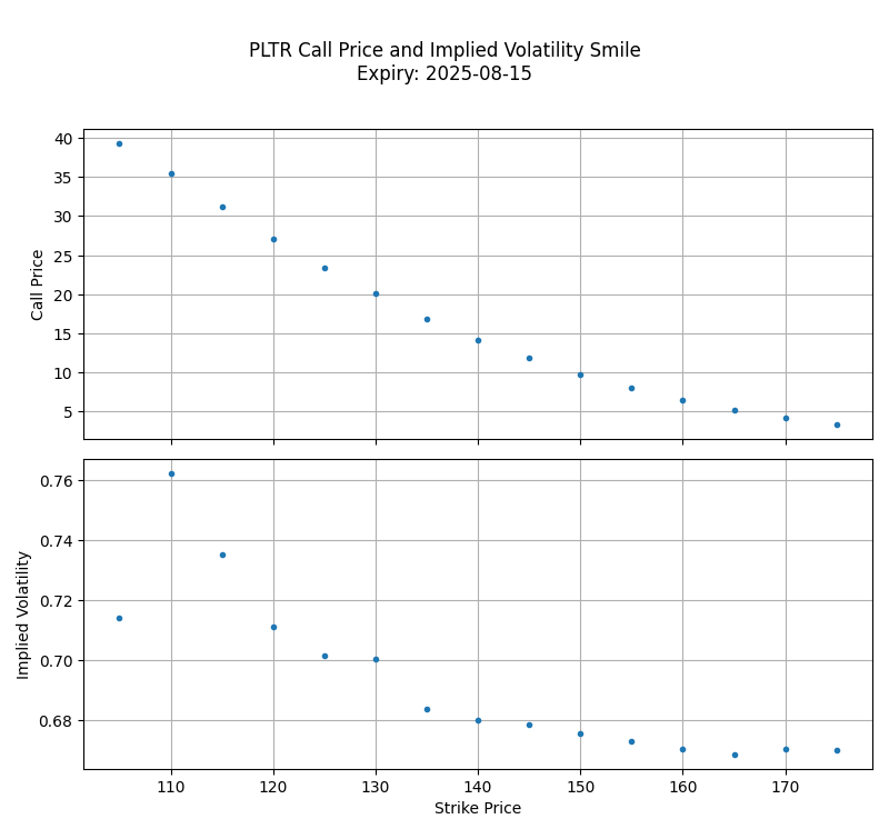
Calculating Implied Volatility

Markets do not quote volatility directly; instead, they quote option prices. Implied volatility (IV) is the volatility that, when plugged into the Black-Scholes formula, gives a model price equal to the market price:

def bs_iv(price, S, K, t, r=0, initial_guess=0.7):
    iv = initial_guess
    for _ in range(1000):
        diff = price - call_value(S, K, iv, t, r)
        if abs(diff) < 1e-4:
            return iv
        iv += diff / call_vega(S, K, iv, t, r)
    return iv

Implied volatility is a standardized measure of market expectations of future volatility. We extract it from market prices to construct the volatility smile, which is crucial for smoothing and differentiating option values later.

Fetching and Preparing Market Data

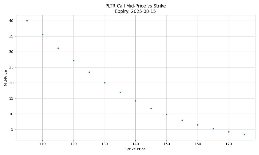
We fetch real market option chains from Yahoo Finance. Each strike has a bid and ask price; we take the midprice as a more accurate estimate of the fair value:

def get_chain(ticker, expiry, min_strike, max_strike):
    opt = yf.Ticker(ticker)
    chain = opt.option_chain(expiry).calls
    chain['midprice'] = (chain.bid + chain.ask) / 2
    return chain[(chain.strike >= min_strike) & (chain.strike <= max_strike)]

To compute PDFs, we need a smooth curve of option prices across a wide range of strikes. We select a strike range that includes both in-the-money and out-of-the-money options for better curvature.

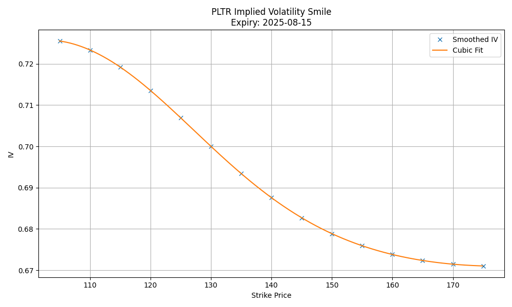
Figure_1 Call Option Mid-Price vs. Strike.png

Figure 1. Call Option Mid-Price vs. Strike.

Building the Volatility Smile

Market IVs vary by strike, creating a pattern known as the "volatility smile." To apply derivatives, we must first smooth the IV curve:

from scipy.ndimage import gaussian_filter1d
from scipy.interpolate import interp1d

def smooth_vol_smile(strikes, iv, sigma=3):
    iv_smoothed = gaussian_filter1d(iv, sigma)
    return interp1d(strikes, iv_smoothed, kind='cubic', fill_value='extrapolate')

Figure_2 Call Price and Implied Volatility Smile.png

Figure 2. Call Price and Implied Volatility Smile.

Smoothing is critical because numerical differentiation is highly sensitive to noise. A clean, smooth volatility smile leads to accurate second derivatives of call prices, and hence accurate PDFs.

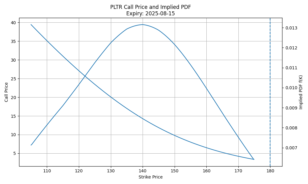
Figure_3 Smoothed Implied Volatility Smile with Cubic Interpolation.png

Figure 3. Smoothed Implied Volatility Smile with Cubic Interpolation.

Extracting the PDF

Once we have a smoothed volatility function, we compute theoretical call prices across strikes, then apply finite differences to approximate the second derivative:

def compute_pdf(S, r, t, strikes, vol_smile):
    C = call_value(S, strikes, vol_smile(strikes), t, r)
    first_deriv = np.gradient(C, strikes)
    second_deriv = np.gradient(first_deriv, strikes)
    return np.exp(r*t) * second_deriv

This is the core of the Breeden–Litzenberger result: second derivatives of call prices give us the implied PDF. This step translates smoothed volatility into actionable probability distributions.

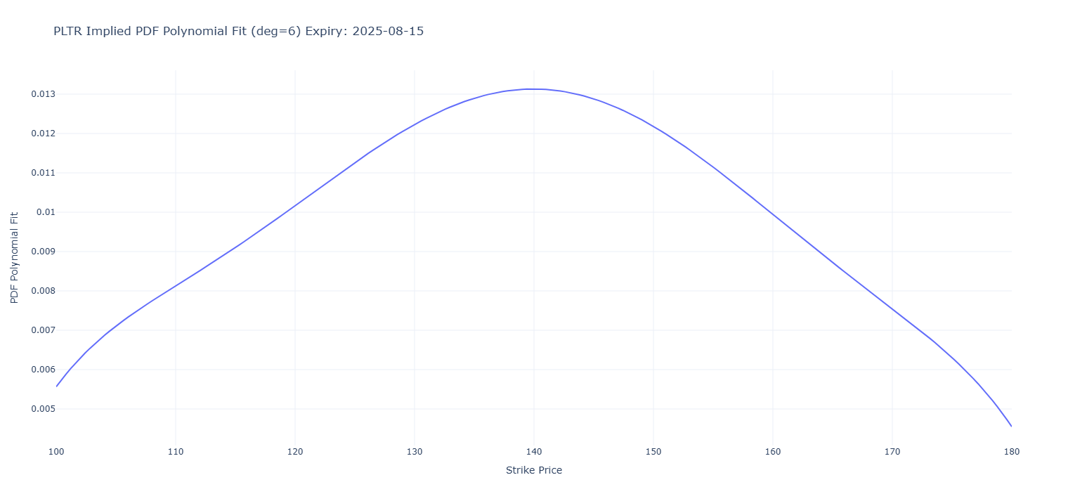
Practical Application: A Case Study on PLTR

We now apply all previous steps to real data for Palantir Technologies (PLTR):

TICKER = 'PLTR'
expiry = yf.Ticker(TICKER).options[5]
min_strike, max_strike = 100, 180

chain = get_chain(TICKER, expiry, min_strike, max_strike)
S = yf.Ticker(TICKER).history(period='1d')['Close'].iloc[-1]
t = (pd.Timestamp(expiry) - pd.Timestamp.today()).days / 365

chain['iv'] = chain.apply(lambda row: bs_iv(row.midprice, S, row.strike, t), axis=1)
vol_smile = smooth_vol_smile(chain.strike.values, chain.iv.values)

strike_grid = np.linspace(min_strike, max_strike, 200)
pdf_values = compute_pdf(S, 0, t, strike_grid, vol_smile)

This section demonstrates the entire workflow on a real-world example, bridging the gap between theory and practical implementation.

Figure_4 Call Price and Extracted Implied PDF via Breeden–Litzenberger.png

Figure 4. Call Price and Extracted Implied PDF via Breeden–Litzenberger for Palantir.

Interactive Visualization with Plotly

To make the output more insightful, we visualize the PDF interactively:

import plotly.graph_objects as go
fig = go.Figure()
fig.add_trace(go.Scatter(x=strike_grid, y=pdf_values, mode='lines', name='Implied PDF'))
fig.update_layout(title='PLTR Implied PDF', xaxis_title='Strike Price', yaxis_title='Probability Density')
fig.show()

Visualizing the PDF reveals the most likely outcomes and the shape of market sentiment, including asymmetry and tail risk.

implied PDF polynomial fit.png

Figure 5. Implied PDF polynomial fit for Palantir at 2025/08/15 expiration.

Interpretation and Applications

With the implied PDF in hand, we can interpret:

Mode (Peak): The most likely future price.
Skew: Bullish or bearish bias.
Tails: Probability of large moves (e.g., crashes or rallies).

This distribution is invaluable for:

Risk management
Pricing structured products
Forecasting market sentiment
Strategy development

Advanced Considerations

Data Quality: Outliers and stale quotes can distort results.
Real vs. Risk-Neutral PDFs: Risk-neutral PDFs must be adjusted for real-world expectations.
Multiple Expiries: Comparing PDFs across maturities reveals how expectations evolve over time.

Conclusion

The extraction of market-implied PDFs transforms raw option data into deep probabilistic insight. By carefully smoothing volatility, applying robust differentiation, and visualizing the output, we uncover the market's view of the future.

This method equips analysts with a quantitative lens to interpret sentiment, manage risk, and develop more informed trading strategies. The power of market-implied PDFs lies not only in their elegance but in their practicality across financial disciplines.

Ready to learn more?

Test our AI powered app by clicking on the top page Launch App button.

Good luck, and happy investment!